There are two types of people coming out of university: managers and specialists. Whilst specialists focus on a single skill, managers need a basic level of expertise in a wide range of skills. This is the first article in a series about elaborating skills which are essential for every manager. Not solely for the purpose of being able to apply these skills directly but for managerial understanding. In this part we will go through one of the most game changing statistic skills: Forecasting
What is forecasting?
Forecasting has been around, as far as can be found in literature, since 44 B.C. Cicero’s well known book “De Divinatione” already stated the importance of the foresight and knowledge of future events. Although it has been around for multiple thousands of years some still do not know of its use. So why should a company use forecasting and why should you know about it? The essence of forecasting is to predict important parameters such as supply, demand or price. These parameters have a direct effect on customer satisfaction as you have to be able to provide the product they want, when they want at the right price. Any help in predicting the amount of product you have to keep in stock to meet supply saves you stress, costs and angry customers. Application examples of forecasting thus include:
- Reducing inventory stockouts
- Scheduling production more efficiently
- Lowering safety stock requirement
- Foreseeing price fluctuations
- Expecting raw material availability
The questions which remains however, is how to actually forecast? To answer that question the different general types of forecasting have to explained. There are a multitude of forecasting techniques which can be divided in three main categories: Judgement, time series and causal forecasting. Judgement forecasting is exactly what the name says: a number of people using their expertise to foresee changes. Judgement is an inaccurate way of forecasting which is often overly optimistic and biased whilst also being heavily reliant on gut feeling and domain knowledge.
Time series forecasting a more well known method, it uses techniques such a exponential smoothing and (weighted) moving averages to get an accurate prediction based on historical data. It has the advantage of being simple to understand and works rather well when demand is stable. Even so, the disadvantages of this type of forecasting are that it is only for short term, it requires lots of historical data and has large errors in volatile markets. The last forecasting type is causal forecasting, a well known concept to everyone with statistic experience as it is focussed on multiple types of regression. This has the advantage of being more accurate than time series and is suitable for medium term forecasting. However, this too has negative aspects: it is expensive, uses even more data than time series and is more complex. This article will focus on time series forecasting, which is something that can be tested at home and will provide a basic intuitive feeling for all other types of forecasting.
Data preparation
When you start forecasting there are essentially two ways to go: you can either use all your raw data and start forecasting or you can prepare your data. Preparing data means reducing the random variation in the observations which exposes the structure of the underlying causal processes. A well known way to do this is by using a rolling average, this article uses the 3mma (three months main average) and 2mma to explain how this works. The 3mma averages the data of three months to take out the random variation in a series of data. This is done with the following formula: \large 3mma=\frac{1}{3}x_{t-1}+\frac{1}{3}x_{t}+\frac{1}{3}x_{t+1}
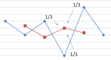
Figure 1. 3mma
The 2mma uses a similar way of thinking, but uses a different as it requires an even number of months. The formula is:\large 2mma=(\frac{1}{2}x_{t-1}+\frac{1}{2}x_{t}+x_{t+1})/2
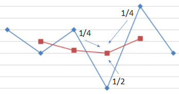
Figure 2. 2mma
The 3mma is simply the average of three months and if you for some reason want to use a 5mma you can just use the average of five months. A 4mma is different and will look like this: \large 4mma=(\frac{1}{2}x_{t-2}+x_{t-1}+x_{t}+x_{t+1}+\frac{1}{2}x_{t+2})/4 This same expanding methodology it can be used on all other even mma types. The reason you want to choose an mma with a higher amount of months is to get a smoother line but remember: the higher the number of months, the less accurate the eventual data. Remember to find the balance between the two as you want to remove any random variation in historical data whilst keeping the accuracy as you are going to use this data to forecast.
Forecasting techniques
You prepared your data, or you didn’t, and you are ready for the real deal. As said before there are numerous forecasting techniques and many companies either created their own, outsourced forecasting or use basic forecasting techniques. Today we’ll focus on three of those basic forecasting techniques: Simple Moving Average (SMA), Single Exponential Smoothing (SES) and Double Exponential Smoothing (DES). Key for deciding on a forecasting technique is to use the simplest technique; if it does not work good enough, move one step up.
The SMA’s formula: \large St = \sum_{i=1}^n (x_{t-k}+ x_{t-k+1}+…+ x_{t})/k. Where:
st = average
k = number of observations
x = Actual
The SMA is one of the most simple and effective forecasting methods, using historical data to predict the average which is used as a forecast for the next month. The effect of more observations means more smoothing and more time lagging. Time lag is a difference or delay between the data and the prediction. Another negative aspect of forecasting is an occurrence called overshooting, which affects linear forecasts. This can be seen in the graph where the turning points of the forecast and the original data are not in the same month. For accurate forecasts you want to reduce the amount of lagging and overshooting.
The next forecast methodology is called SES, which is similar to a weighted moving average with exponentially decreasing weights. It uses the following formula: St = α*x_ {t} + (1-α)*S_{t-1}. Where:
α = data smoothing factor
0 < α < 1
S = Estimated level = Forecast
x = Actual
This formula is used for short term linear forecasting and the amount of smoothing in this forecast can be changed by the size of the alpha. The lower the alpha, the higher the smoothing but also the higher the amount of lag and the amount of overshooting. There are also a double and a triple version which take into account trending as well as seasonality but those are left out of this article due to them being to advanced. SES and trends are both moving averages, with weights exponentially decreasing over time. For this formula, the smaller α and β are the more smoothing, but as it is linear it will result in time lagging and overshooting. The previously noted forecasts are a great way to get a feel for forecasting and the essential parts of it. They are however, not the most advanced possibilities as there are still many other techniques. The hardest forecasting techniques all include the key elements of a forecast: trends, seasonality, cycle, causal factors and other unexplained variance. As you might have noticed, the methods thus far have only used a max of one of these elements. As such there are a lot more techniques to use with the most modern techniques including demand modelling and machine learning to improve accuracy and reduce error margins.
Bullwhip effect
Forecasting might sound nice and without any major risks. However, there are certain cases where you will have to really think about the accuracy of your forecast. An example of this is the well studied bullwhip effect. The bullwhip effect is a distribution channel phenomenon in which forecasts disrupt supply chains. It refers to increasing swings in inventory in response to shifts in customer demand as one moves further up the supply chain. In simple words this means that if consumer demand suddenly rises, a retailer will raise demand, the supplier will raise demand and so on. Keep in mind that this rise will happen exponentially, leading to greater safety stocks, inefficient production or excessive inventory. Whilst there are multiple countermeasures intended to reduce uncertainty and variability, the best method to prevent this is to look at your forecast and recognize changes that seem unnatural or should not occur.
Sources:
http://www.flostock.nl/index.php?id=892
Robert Peels (Flostock) – Lecture on Bullwhip effect
http://www4.hcmut.edu.vn/~ndlong/QLXD-HD/mat/05_The_Bullwhip_Effect_in_Supply_Chains.pdf
https://pdfs.semanticscholar.org/1edf/af279f01d6ea3469b20c57cff6fa69dec219.pdf

0 Comments